Taking a look under the hood of the self-attention mechanism!#
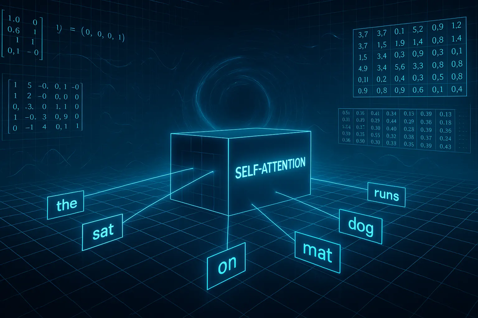
The goal of self-attention is to identify and weight the mutual dependencies between tokens in the sentence context.

For each individual token, a new context-adjusted embedding is calculated – that is, a new embedding vector that takes into account the weighted information from all tokens up to the current token in the sentence.
This way, a new representation is created for each token, which reflects its meaning in the context of the other tokens.
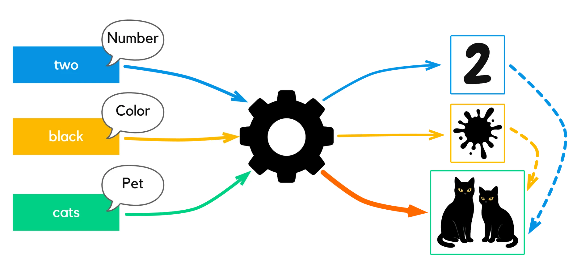
Each token starts with its own embedding from the raw embedding lookup table – this is learned during training and remains unchanged during inference. For example, “two” can be represented as a number, “black” as a color, and “cats” as a pet.
Through the transformer mechanism, these pieces of information are processed together. As a result, the token “cats” receives a new, context-adjusted embedding that reflects the meaning of the entire sentence – the image of two black cats. (Real embeddings are, of course, latent, as we have already seen.)
A transformer performs a large number of computations – and does so simultaneously for many tokens.
To carry out all these computations – from the Q/K/V transformations to the weighting of context information – efficiently, it needs a tool that can perform many operations in parallel and at lightning speed.
➔ This is where matrices come into play …
Math? Don’t worry!#
To truly understand self-attention, we need a bit of math – but don’t worry, it’s manageable and intuitive.
The two most important tools are:
Vectors: Lists of numbers (we already know these)
[0.3, -1.2, 4.7, ...]
Matrices: Tables of numbers – they enable fast, parallel computations
[ 1  2  3 ]
[ 4  5  6 ]
[ 7  8  9 ]
Why Matrices?#
The groundbreaking publication by Vaswani et al. (“Attention Is All You Need”) not only introduced a revolutionary architecture but also built it entirely on matrix operations.
This approach remains at the core of modern transformer models to this day – including GPT, Claude, Gemini, Granite, and many others.
Since then, the computational structure has only been slightly optimized, but the basic idea has been carried over almost unchanged.
Why Matrices are so powerful#
Matrices have two key advantages:
- They make it possible to perform millions of mathematical operations in a single step – thanks to highly optimized matrix multiplication.
- They are perfectly suited for parallelization on GPUs – which makes them ultra fast.
Matrices have been used in computer graphics for decades – especially in an area almost everyone knows: 3D games.
In recent years, the quality and realism in games have literally exploded.
The main reason: graphics cards (GPUs) have become increasingly powerful and can perform millions of vector and matrix calculations per second.
You could say: power gamers paved the way, making today’s computers true matrix specialists – a development from which AI models benefit massively today.
Experience Matrices in action!#
In this 3D scene, you see a spaceship as a vivid example.
One matrix is enough
Instead of performing each calculation step – such as translation, rotation (around the X, Y, and Z axes), scaling, etc. – individually, the entire model including its environment is transformed with a single so-called model-view-projection matrix (MVP).
Different Perspectives
You can view the spaceship from different perspectives – similar to how we later apply transformations to embeddings in order to capture information from various viewpoints.
👉 Try it out: You can move freely in the scene using your mouse or touch!
- Left mouse button: rotate,
- Right mouse button: pan,
- Scroll wheel: zoom.
Three different views of each token#
Each token originally exists as an embedding vector – a vector with, for example, 12,288 numbers that represent its meaning in a high-dimensional space.
From this embedding vector, three new vectors are formed through projection, each serving a different function in the attention mechanism:
- ❓ Query (Q) vector – compared with the keys of the other tokens for similarity
- 🔐 Key (K) vector – serves as the basis for this comparison
- 📦 Value (V) vector – whose contents, depending on relevance, flow into the new representation of the token
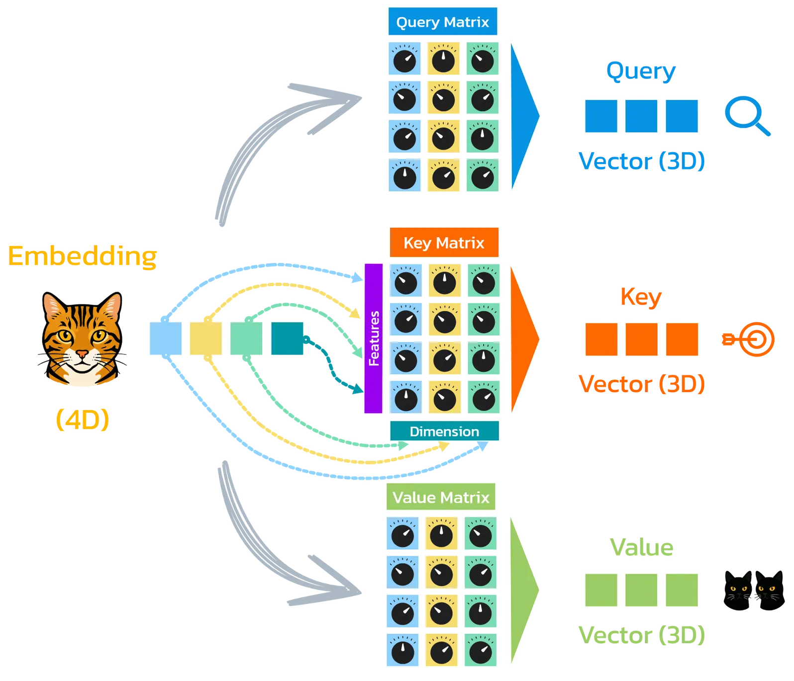
The transformation is carried out by three different weight matrices – learned during training with billions of words:
One for query, one for key, and one for value.
Quick excursion into multiplying matrices and vectors:
When you multiply a vector by a matrix, you go column by column through the matrix: you multiply each element of the vector by the element in the same row of that column, add up the products – and these sums are the entries of the new vector.
The length of the vector must match the number of rows of the matrix.
The calculation steps are simple – I’ve written them down for you here:$$ \vec{v} \cdot W = \begin{bmatrix} \color{blue}{2} & \color{red}{3} & \color{green}{1} & \color{orange}{1} \end{bmatrix} \cdot \begin{bmatrix} \color{blue}{1} & \color{blue}{0} & \color{blue}{2} \\ \color{red}{2} & \color{red}{1} & \color{red}{1} \\ \color{green}{0} & \color{green}{1} & \color{green}{0} \\ \color{orange}{1} & \color{orange}{0} & \color{orange}{1} \end{bmatrix}= \begin{bmatrix} \color{blue}{9} & \color{red}{4} & \color{green}{8} \end{bmatrix} $$
$$ \color{blue}{2} \cdot \color{blue}{1} + \color{red}{3} \cdot \color{red}{2} + \color{green}{1} \cdot \color{green}{0} + \color{orange}{1} \cdot \color{orange}{1} = 2 + 6 + 0 + 1 = \color{blue}{9} $$ $$ \color{blue}{2} \cdot \color{blue}{0} + \color{red}{3} \cdot \color{red}{1} + \color{green}{1} \cdot \color{green}{1} + \color{orange}{1} \cdot \color{orange}{0} = 0 + 3 + 1 + 0 = \color{red}{4} $$ $$ \color{blue}{2} \cdot \color{blue}{2} + \color{red}{3} \cdot \color{red}{1} + \color{green}{1} \cdot \color{green}{0} + \color{orange}{1} \cdot \color{orange}{1} = 4 + 3 + 0 + 1 = \color{green}{8} $$
For each token, the original embedding x_i is multiplied by the three weight matrices
W_Q, W_K, and W_V to generate the three vectors query (Q), key (K), and value (V).
These form the basis of the self-attention mechanism – relying entirely on matrix operations and therefore highly efficient.
In practice, there is an additional advantage: all tokens of the input sequence X are processed in parallel – through a single matrix multiplication, where each row corresponds to a token.
$$ \begin{aligned} \mathbf{Q} &= \mathbf{X} \cdot \mathbf{W}^Q \\ \mathbf{K} &= \mathbf{X} \cdot \mathbf{W}^K \\ \mathbf{V} &= \mathbf{X} \cdot \mathbf{W}^V \end{aligned} $$
The weight matrices have as many rows as the embedding has dimensions (e.g., 12,288) and as many columns as the desired target dimension specifies (e.g., 128).
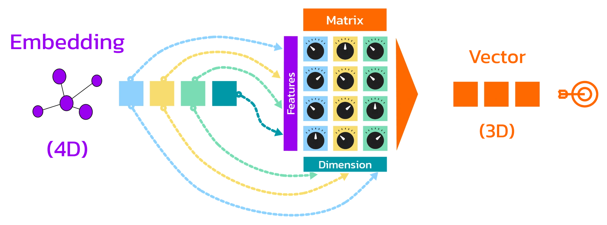
The embedding is multiplied elementwise with each column of the weight matrix and the products are added:
- The first column yields the first new feature,
- the second column yields the second new feature,
- and so on …
Each of these new features is created through a linear projection of the original features – some are amplified, others diminished, some completely filtered out, or even reversed (negated).
In this way, the original feature vector is transformed into a new representation in a more compact, reduced feature space – for example, from 12,288 to 128 features.
Important to emphasize again!#
- All tokens use the same Q, K, and V matrices per attention head.
There are no token-specific weightings; instead, there is a uniform transformation for all inputs – ensuring maximum efficiency and generalization. - The Q, K, and V matrices are independent of each other.
They cannot be derived from or directly related to one another – each has its own parameters, which are learned exclusively through training. - With such a Q/K/V projection, the model can capture only one specific type of semantic relationship between tokens.
A single attention head typically represents exactly one perspective – for example, “which subject belongs to which verb?”. - In a complete transformer model, however, multiple heads operate simultaneously and across multiple stacked layers.
This creates thousands of projections, which together capture a wide range of semantic patterns and dependencies – from sentence structure to meaning across entire paragraphs – more on that in a later section.
Why is the dimension reduced?#
- The reduction saves computation time and memory – especially with large context sizes,
since the calculations in the attention mechanism increase quadratically with the number of tokens. - It allows the model to represent information in a more compact form –
each so-called attention head thus works with its own projection, which can highlight specific aspects of the original features. - The transformer uses multiple such attention heads.
For each head to work efficiently, the original embedding dimension is split – e.g., with 96 heads: 12,288 / 96 = 128 dimensions per head.
👉 In this interactive demo, the principle is vividly visualized#
How are these Q, K, V matrices created?#
The Q, K, and V matrices are learned through training on massive amounts of text – usually billions of words.
The training objective is always the prediction of the next token.
-> Incorrect predictions lead to feedback via backpropagation.Through this process, the matrices learn to:
- Adjust query and key vectors so that relevant tokens show high similarity to each other
- Shape value vectors so that only context-relevant information is passed on
How the transformer recognizes which tokens are relevant to each other#
In the chapter on embeddings, we already saw that semantically similar tokens are located closer together in the embedding space.

The closeness of two vectors is measured either by their distance or the angle between them – in some methods, their length also plays a role.
In transformers, it is primarily the angle between the vectors that plays a central role – not their Euclidean distance.
As a reminder: there are two common methods to measure similarity via angles:
Scalar Product (Dot Product)
Here, the corresponding components of two vectors are multiplied and then summed up.
The result is a single value that expresses semantic similarity:
- close to 0 → little similarity
- positive → semantically similar
- negative → rather opposite
$$ \mathbf{x} \cdot \mathbf{y} = \sum_{i=1}^{n} x_i , y_i $$
Cosine Similarity
Cosine similarity is a normalized dot product.
It considers only the angle between the vectors – independent of their length.
The result is always between –1 and 1.
$$ \cos(\theta) = \frac{ \vec{A} \cdot \vec{B} }{ | \vec{A} | \cdot | \vec{B} | } $$
| Value | Meaning |
|---|---|
| +1 | exactly the same direction |
| 0 | orthogonal → no similarity |
| −1 | exactly opposite |
Attention Attention!#
In transformers, what is crucial is which tokens influence one another.
More precisely: for each individual token, what matters is how relevant the other tokens are to it — that is, what information they can contribute to its representation in context.
To calculate this relevance, we have already projected the tokens differently using the weight matrices:
Once as a query vector and once as key/value vectors.
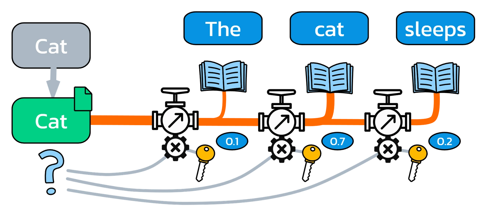
The better a token’s ❓query matches the 🔐keys of the others, the more 📦value is taken from those tokens.
Attention Score#
The calculation of attention between tokens is called the attention score.
This is not about a classic geometric distance, but rather a measure of their closeness in embedding space – for example, via cosine similarity.
Vaswani et al. chose the pragmatic solution, which is particularly efficient:
Instead of calculating the more complex cosine similarity with additional normalization,
they directly use the dot product:
$$ \text{score} = \mathbf{q} \cdot \mathbf{k}^\top $$
The dot product has another advantage:
In the dot product, both the angle between the vectors and their length contribute to the result.
This gives the model the freedom to take into account both the direction (semantic closeness) and the magnitude of individual features (vector lengths).
However, this creates a small problem:
Dot products in high-dimensional spaces can take on very large values.
This makes later weighting more difficult, because some tokens would be emphasized excessively, while others would hardly be considered at all.
The solution is simple and efficient:
Divide the result by the square root of the dimensionality of the key vector (√dₖ).
This keeps the scores stable and comparable:
$$ \text{score} = \frac{\mathbf{q} \cdot \mathbf{k}^\top}{\sqrt{d_k}} $$
👉 Token Relevance: Try out how angles and dimensions affect cosine similarity and the dot product#
What does the T in the keys mean?
The ‘T’ stands for transpose: it turns the key row vector into a column vector so that the dot product with the query row vector can be computed.
The Attention Score Matrix#
Now we calculate these scores for all possible combinations of tokens in the sentence context.
To do this, we create a table: all tokens appear both in the rows (as query) and in the columns (as key).
At each intersection, the dot product between the query vector and the key vector is computed – this yields the attention score.
This results in a complete attention matrix that shows how strongly each token attends to all the others.(In this attention matrix, only positive scores appear, although negative ones would also be possible.)
The attention score matrix is conceptually of size n × n. The computational cost therefore grows quadratically with the length of the context window, and with a “naïve“ implementation this also applies to memory usage.
At several thousand tokens, the required resources increase significantly and quickly push current hardware toward practical limits. Without special optimizations, only a few thousand tokens can typically be processed efficiently in practice.
Very large context windows on the order of 100,000 tokens and beyond are technically possible, but require optimized approaches such as FlashAttention as well as, in some cases, additional structural methods like sparse attention or segmentation.
Another limiting factor is the attention mechanism itself — with very long contexts, the focus can become so widely distributed that important parts lose weight.
In practice, attention scores are computed as a scaled matrix product of the query matrix and the transposed key matrix. Modern implementations such as FlashAttention perform this computation block-wise (tiled) and avoid storing the full n × n score matrix in memory. $$ \text{score} = \frac{\mathbf{Q} \cdot \mathbf{K}^\top}{\sqrt{d_k}} $$ (Vectors are usually written in lowercase (for example: q, k, v), while matrices are written in uppercase (for example: Q, K, V).)
Now the real values matter!#
In the next step, the value vectors finally come into play.
Now it is determined which information from the context is transferred to which token.
But before we begin, we still need to solve one problem …
please don’t cheat …#
If we take into account all attention scores in the sentence for each token, the model could also access tokens that only come later – and thus use information that it shouldn’t actually know at that point.
This contradicts the idea of an autoregressive decoder, which is only allowed to access previous tokens when making predictions.
The Attention Mask#
How do we prevent this cheating?
With a simple trick: we use a mask.
All scores that refer to future tokens are masked out – or more technically:
They are replaced with −∞ (or a very large negative number) so that these positions are completely excluded from the calculation.
When weighting (softmax) is then applied, these positions are automatically set to zero – and thus completely ignored.
How much does each token contribute?#
With the attention matrix, we now know which tokens pay attention to each other. But how exactly do these scores influence which features a token takes over from others?
The central idea: in context, tokens don’t just receive attention, they also adopt features – specifically from the value vectors of the tokens they focus on.
The team around Vaswani developed an elegant mechanism for this:
You go row by row through the attention matrix – that is, token by token – and calculate for each target token how strongly the other tokens in the row contribute.
However, the raw attention scores are not directly suitable for computation – they are not scaled, not normalized, and difficult to compare.
That’s why we need a function that brings order to these values and allows us to weight them reliably.
The Role of the Softmax Function#
This is where the softmax function comes into play.
It is a mathematical method that can transform a list of numbers into relative weightings.
Each value is first amplified by the exponential function and then normalized so that all results lie between 0 and 1 and their sum equals exactly 1.
This creates proportional weightings: larger input values receive more weight, smaller ones less – thus the selection is directed specifically toward the most relevant tokens.
The softmax function thus provides us, for each token in an attention row, with exactly the multiplier by which its value vector is weighted into the target token.
The softmax values of a row always add up to exactly 1 – ensuring that the resulting combination of value vectors is stable and balanced.
$$ \text{Softmax}(z_i) = \frac{e^{z_i}}{\sum_{j=1}^{n} e^{z_j}} $$
👉 Try out how the softmax weightings change when you adjust the score values:
The New Embedding Emerges#
Now we have everything together:
- The attention matrix shows how strongly a token attends to others.
- The softmax function converts these values into weightings.
- The value vectors contain the features that are passed on.
Now we calculate, for each token, the weighted sum of the value vectors – using the softmax values as multipliers.
The result is a new, context-sensitive feature vector – in other words, the new embedding.
This vector summarizes which information from the entire sentence context is important for the current token.
The Formula That Is Changing the World!#
$$ \cancel{\boldsymbol{E = mc^2}} $$
$$ \mathbf{Attention}(\mathbf{Q}, \mathbf{K}, \mathbf{V}) = \mathbf{softmax}\left( \frac{\mathbf{Q}\mathbf{K}^\top}{\sqrt{d_k}} + \mathbf{M} \right)\mathbf{V} $$
The entire process of self-attention, which we have described here, was summarized by Vaswani and his team in a single elegant formula.
All respect for this brilliant mechanism – to Vaswani, the entire research team, and of course also to all those who paved the way beforehand.
In today’s tools like ChatGPT, Gemini, and many others, we see developments that just a few years ago we would have considered unthinkable.
And it is very likely that we will soon witness further emergent phenomena – developments that will not only challenge our current imagination but far exceed it.
What’s Next?#
With self-attention, we have now created an embedding that takes into account the entire context for each token – especially the last one (“sleeping”).

What’s still missing: this embedding must be assigned to a specific next token.
For this, another neural network comes into play: a feedforward layer, which further processes the embedding – and helps to recognize logical and semantic patterns.
In the end, a decoder generates a probability distribution over the vocabulary – and selects the most likely next token.
How this works, we will see in the next chapter.
© 2025 Oskar Kohler. All rights reserved.Note: The text was written manually by the author. Stylistic improvements, translations as well as selected tables, diagrams, and illustrations were created or improved with the help of AI tools.