The major advantages of modern transformer models#
The three most important advantages of current LLMs with transformer architecture:
- Parallel processing: All tokens are processed simultaneously – not step by step.
- Better text understanding: The model recognizes complex semantic relationships.
- Long context: Transformers can consider thousands of tokens at the same time
These advances enable applications that were completely unthinkable just a few years ago.
How Much Text Does a Language Model Really Understand?#
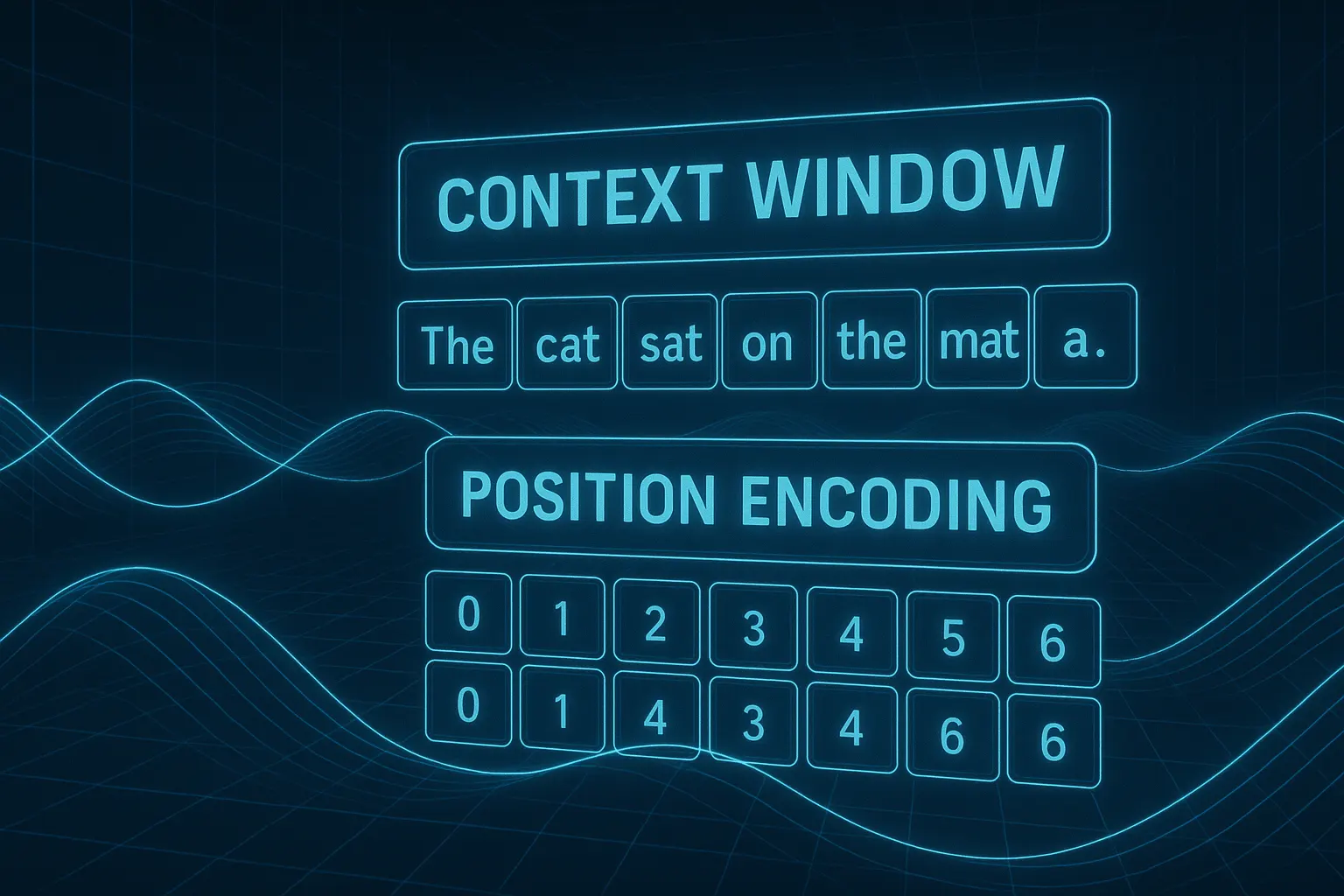
The length of the so-called context window is a central aspect of modern language models.
An LLM analyzes all tokens in the context window simultaneously and relates them to one another. This way, it can “understand” the entire text.
The larger this window, the more text the model can capture at once – not just individual words and sentences, but even entire sections or chapters.
The size of the context window largely determines the application scope of a language model – and is therefore a decisive competitive factor in the development of powerful LLMs.
In recent years, the maximum context length has increased massively:
| Modell | Kontextfenster (Tokens) | Ca. Seiten | Jahr | Anbieter |
|---|---|---|---|---|
| GPT-1 | 512 | < 1 | 2018 | OpenAI |
| GPT-2 | 1.024 | ~1,5 | 2019 | OpenAI |
| GPT-3 | 2.048 | ~3 | 2020 | OpenAI |
| GPT-3.5 | 4.096 | ~5–6 | 2022 | OpenAI |
| GPT-3.5 Turbo | bis 16.384 | ~20–25 | 2023 | OpenAI |
| GPT-4 | 8.192 / 32.768 | ~10 / ~40 | 2023 | OpenAI |
| GPT-4 Turbo | 128.000 | ~160 | 2023 | OpenAI |
| Claude 1 | ~9.000 (estimated) | ~12 | 2023 | Anthropic |
| Claude 2 | 100.000 | ~130 | 2023 | Anthropic |
| Claude 3 | 200.000 | ~260 | 2024 | Anthropic |
| Gemini 1.5 | 1.000.000 | ~1.300+ | 2024 | Google DeepMind |
| LLaMA 2 | 4.096 | ~5–6 | 2023 | Meta |
| LLaMA 3 | 8.192 – 32.000 | ~10–40 | 2024 | Meta |
| Mistral 7B | 8.192 | ~10 | 2023 | Mistral.ai |
| Mixtral (MoE) | 32.768 | ~40 | 2023 | Mistral.ai |
| Command R+ | 128.000 | ~160 | 2024 | Cohere |
The table clearly shows: some models have expanded the context window almost explosively.
However, this increase is often achieved through technical workarounds or memory tricks – because in reality, the effectively usable context depth for most models still lies in the range of a few thousand tokens.
But – where exactly is each token located?#
Parallel processing brings with it a problem that serial models like RNNs do not have:
The order of the tokens in the context.
Example:
- The dog bit the mailman.
- The mailman bit the dog.
Both sentences contain exactly the same words – but the order of the words completely changes the meaning.
Transformers therefore need to know: At which position is each token located?
This problem was also clear to Vaswani and his team:
A transformer processes all tokens simultaneously – but does not know the order in which they appeared in the sentence.
Therefore, a method had to be found to provide the model with positional information:
It needs to know at which position in the sentence a token originally appeared.
Positional Encoding#
For this, each token is assigned a positional indicator.
This can either be done statically – using a fixed number for each position –
or the model can learn on its own how to remember the position – using an internal table.
But the problem is a bit more complex than it first sounds:
It is not enough to simply assign a number to the token – such as position 1, 2, 3 …
because the position must also be reflected in the embeddings, i.e., in the individual feature dimensions that the model processes internally.
Only then can the model learn how semantic relationships change when the tokens appear in different positions in the sentence.
For this, Vaswani chose a very elegant solution:
The so-called sinusoidal position encoding – also known as the “Vaswani method”.
“Vaswani Method”#
The idea:
Each position in the sentence is converted into different values using sine and cosine functions – separately for each dimension in the embedding.
This creates a unique wave pattern that encodes the position – mathematically distinguishable for each token and each dimension in the embedding.
$$ PE_{(pos, i)} = \begin{cases} \sin\left(\frac{pos}{10000^{\frac{2i}{d}}}\right), & \text{for even } i \\ \cos\left(\frac{pos}{10000^{\frac{2i}{d}}}\right), & \text{for odd } i \end{cases} $$ where:
- ( pos ): position in the sentence
- ( i ): index of the dimension
- ( d ): dimension of the embedding
The exact formula is less important – what matters is:
You can see that the positional encoding varies depending on the position in the sentence and the embedding dimension.
Sine and cosine functions alternate and start with shifted phases – creating a unique, distinguishable wave pattern for each position.
The following interactive graphic shows the positional encoding in detail – you can control and explore it yourself.
The positional encoding is simply added to the token’s vector – i.e., to each individual embedding.
This slightly shifts the position of the token in the feature space, allowing the LLM to recognize where in the sentence the token originally appeared.
Modern methods like RoPE#
Newer models use a refined form of positional encoding – such as RoPE (Rotary Positional Encoding).
Here, the token itself is not shifted in the feature space, but rather the way the token is viewed is slightly rotated.
RoPE is a relative but fixed positional encoding – it integrates the distances between tokens directly into the calculation instead of encoding absolute positions.
The underlying principle, however, remains the same:
The positional information must be provided to the model – otherwise it cannot capture the order of the tokens.
© 2025 Oskar Kohler. All rights reserved.Note: The text was written manually by the author. Stylistic improvements, translations as well as selected tables, diagrams, and illustrations were created or improved with the help of AI tools.